Calculate sterodynamic sea-level patterns from CMIP6 models#
Overview#
The recipe recipe_steric_patterns calculates sterodynamic sea-level change patterns from CMIP6 model datasets. Patterns are calculated for the SSP2-4.5, SSP3-7.0 and SSP5-8.5 scenarios.
These patterns are useful because we can emulate spatially-resolved sterodynamic sea-level rise from global thermal expansion at a fraction of the computational cost of running a fully-coupled Earth system model or ocean model.
The methods for this recipe are derived from those in Palmer et al. (2020) which themselves are rooted in the IPCC AR5 report.
Note
The regrid setting in the recipe is set to a (180, 360) grid to put all models on the same grid.
Available recipes and diagnostics#
Recipes are stored in esmvaltool/recipes/
recipe_steric_patterns.yml
Diagnostics are stored in esmvaltool/diag_scripts/steric_patterns/
steric_patterns.py: generates sterodynamic patterns from input datasets
sub_funcs.py: set of sub functions to assist with the main script
User settings in recipe#
Script steric_patterns.py
Required settings for script
None
Optional settings for script
None
Required settings for variables
short_name
additional_datasets
exp
Optional settings for variables
None
Required settings for preprocessor
regular_grid: regrids data to a (180, 360) grid
Optional settings for preprocessor
None
Variables#
Script steric_patterns.py
zostoga (ocean, monthly, time)
zos (ocean, monthly, longitude, latitude, time)
Observations and reformat scripts#
None
References#
Palmer, M. D., Gregory, J. M., Bagge, M., Calvert, D., Hagedoorn, J. M., & Howard, T., et al. (2020). Exploring the drivers of global and local sea-level change over the 21st century and beyond. Earth’s Future, 8, e2019EF001413. https://doi.org/10.1029/2019EF001413
Perks, R., & Weeks, J. (2023). MetOffice/ProFSea-tool: v1.0.0 (v1.0.0). Zenodo. https://doi.org/10.5281/zenodo.10255468
Example plots#
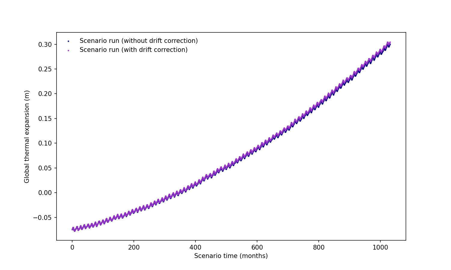
Fig. 364 Detrended zostoga, correcting for model drift using the pre-industrial (PiControl) experiment following Palmer et al., (2020). This is done for each model and scenario.#
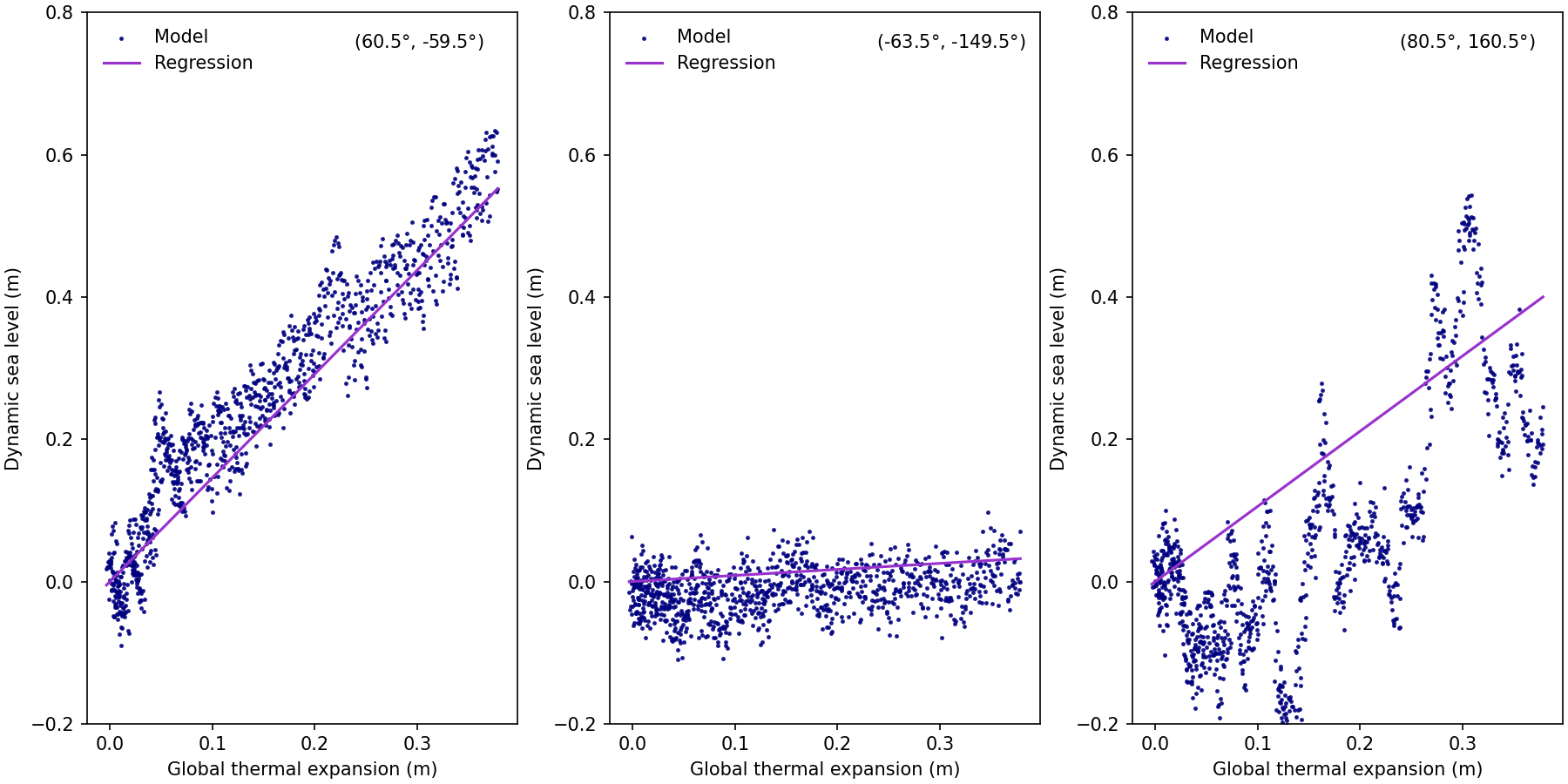
Fig. 365 Example of the regressions between the global thermal expansion (zostoga) and local dynamic sea-level height (zos) for three random grid-cells. The coordinate for each of the grid-cells is shown in the top-right corner of each panel.#
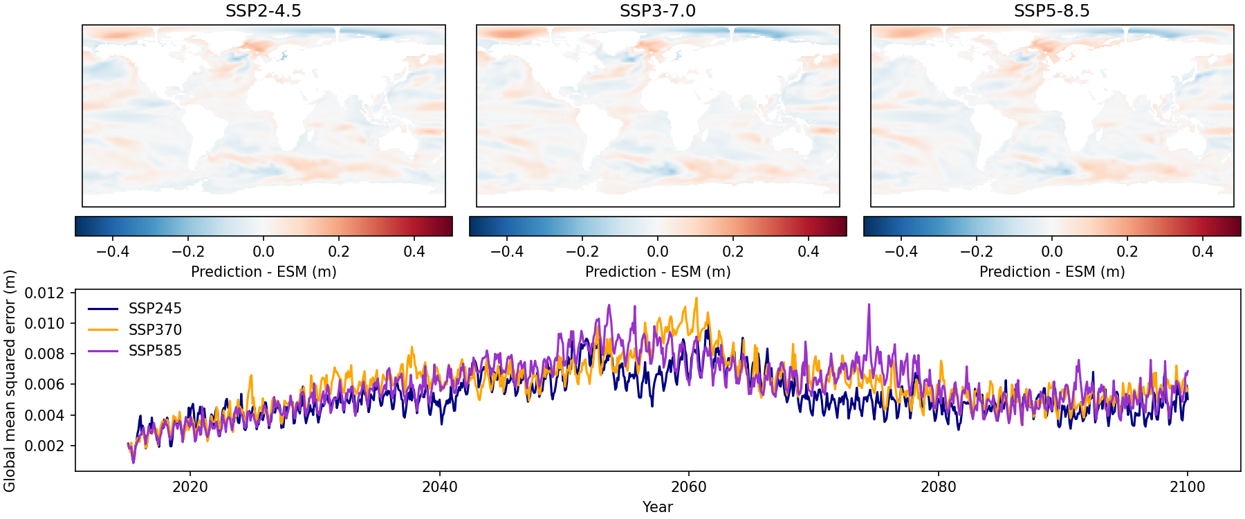
Fig. 366 Example end-of-century predictions from the UKESM1-0-LL model patterns for each SSP, as well as a timeseries of globally-averaged mean-squared error. Two polar artifacts can be seen in each map panel, seemingly occuring due to ESMValTool’s regridding functionality. This seems to occur more often on low-resolution models as opposed to high-res.#